Machine Learning for Game Devs: Part 2

This article is the second of a three-part series on machine learning for game devs. Read Part 1 here.
By Alan Wolfe – SEED Future Graphics Team
Gradient Descent
When we train a neural network, we’re trying to find the weight and bias values that give us the lowest possible cost for all inputs. Cost, in this case, is the “rightness” or “wrongness” of an output’s relationship to an input as measured by a cost function, with low costs being more “right” or favorable.
How do you figure out a neural network’s optimal weight and bias values?
You could…
- Randomly generate many sets of weights and biases, then keep the one that produces the lowest cost. (Probably the one with the lowest sum of squared costs for all inputs.)
- Start with a randomized set of weights and biases, then try to improve it.
Method 1 is fine if you’re working with a small number of weights, but it very quickly runs into problems when dealing with a realistically-sized neural network. Even the simple neural network we’ll be making in Part 3 of this series has nearly 24,000 weights to train! With 10, 50, or 100 neurons in your network, you could get lucky with random weights, but in a larger search space with thousands of neurons, luck isn’t going to get you far.
Method 2, where you start with a random network and work to improve it, is a much better way to go. It’s also what we’ll be talking about from here on.
Rolling a Ball Downhill
Finding the best weights to minimize a cost function is like graphing the cost function and finding the lowest point on the graph. The variable(s) we are graphing are the neural network weights and biases. First-year calculus lets us find the lowest point on graphs for simple functions, but for more complex functions of several variables, it gets complicated. Luckily, there’s a simple solution: Drop a ball at a random point on the graph and let it roll downhill until it reaches the bottom.
If you want to be more confident that you’ve found the lowest point of the deepest valley (the global minimum), you can drop a whole bunch of balls at random and keep the result from whichever ball found the deepest valley (which would be the same as the lowest cost). Ultimately, the goal here is to find the global minimum – without getting stuck in a local minima.
Fortunately (and somewhat confusingly), adding neurons to a neural network makes it easier to find the global minimum. That’s because adding neurons to a neural network also adds weights and biases, making the problem higher dimensional. And in higher dimensions, the chance of getting caught in a local minima goes down.
Think of it as expanding your movement options: Even if you’re stuck in a valley on one axis of the graph, there are plenty of other axes where you aren’t stuck in that valley. Which means that getting out of it can be as simple as rolling to the side.
Following that same line of thought: The more dimensions you can move in, the less likely you are to get stuck, since “stuck” would mean being in a spot where every axis is a valley.
(For more on this topic, check out the Lottery Ticket Hypothesis and the Multi-View Hypothesis.)
Which Way Is Downhill?
One of the most widely used techniques for this dropping-a-ball-downhill approach is ADAM, which adds momentum to the ball (and a few other things) to help it find deeper valleys.
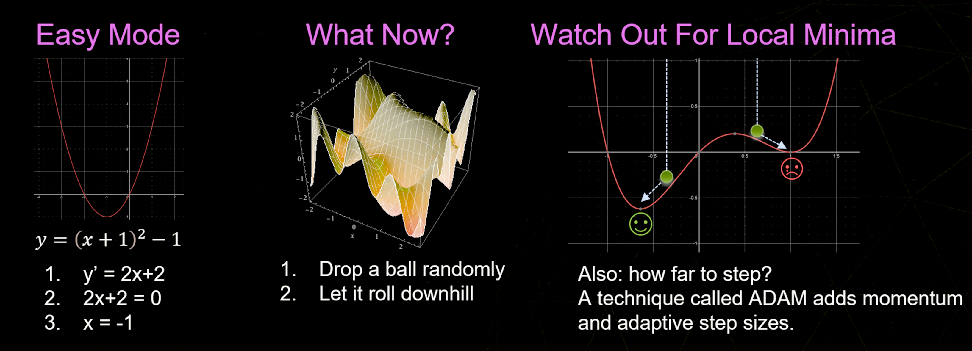
Finding the minimum point on a complicated high-dimensional graph: drop a ball and let it roll downhill.
But even if we know that we should pick a random spot and move downhill, there’s still another question: How do we know which way is downhill? If we had a simple one-dimensional function y = f (x), we could use the slope of the line at a point to know if “downhill” meant going left or right. And if you remember that the slope of a function is the same as its derivative, you can generalize the derivative to higher dimensions and get the gradient.
The gradient has the derivative of each variable (which is the same as each axis) and points in the steepest uphill direction. To find the steepest direction downhill, you just go in the other direction.

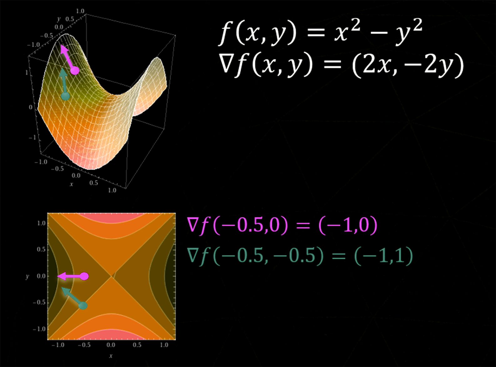
The gradient is the vector that points uphill in the steepest direction.
The gradient is rarely going to be a straight line from where we are to the deepest valley — it’s more likely to be curved and make turns. To handle this, we are going to calculate the gradient, take a small step, calculate the gradient again, take another small step, and keep going until we seem to be at a minimum. The size of the steps we take will be based on the learning rate we mentioned in Part One of this series.
Beyond Neural Networks
Gradient descent isn’t limited to neural networks; it’s a generic optimization strategy for differentiable functions. It even has some tolerance for things not being completely differentiable. Writing differentiable code is actually a lot like writing branchless code because branches are a major source of discontinuities! If you can write code to be (mostly) differentiable, you can use gradient descent to search for a good solution for values of tunable parameters. If you have a cost function that gets smaller for better solutions, it will look for the parameter values with the lowest cost.
Imagine that you have a photograph of an object and you want the mesh of that object. You could start by randomly generating 1,000 randomly-oriented and -colored triangles, plus randomized lighting parameters. You could then render the image and sum up the difference between the pixels in your image and the ground truth. If you took the gradient of that, ending up with a derivative for each randomized parameter (several thousand of them), that would tell you how to adjust all those things to get a little bit closer to the ground truth. Repeat that enough times and you might start to get something that looks like the photograph. You will have reconstructed the object — at least from that one vantage point. But if you move the camera, it might be completely flat in the back or have other problems, because it isn’t defined.
Setting aside some details, this is essentially how NeRFs work.
(By the way, if you ever want to make a differentiable renderer: Geometry edges end up being a large problem to solve, but there’s ongoing research in that area.)
In summary: Gradient descent is used to train neural networks, but it isn’t limited to neural networks. Any differentiable process can use gradient descent to find optimal parameter values for a scoring function.
Of course, coming up with a scoring function that gives you the results you want can be quite a challenge. More often than not it’s like talking to a genie where, sure, you can get what you wish for… but only if you make exactly the right wish.
Three Methods for Calculating Gradients
Now that we’ve defined gradients, let’s look at three different ways to calculate them.
Finite Differences: Easy-Mode Gradients
Let’s start by thinking about derivatives. A derivative dy / dx tells us how much y changes for each step you take on x in a function, y = f (x).
If we want to know how much y changes when we change x, we could simply take a step on x and see how much that changes y. This method of calculating a derivative is called “finite differences,” and we’ll explore two different ways to do it: forward differences and central differences.
Forward Differences
To calculate a derivative using forward differences, you would:
- Take a step forward on x by a value ε (epsilon) to get the difference between the new y value and the old y value.
- Divide that difference by ε to get the derivative.

This equation will give you an exact, correct derivative for a line, but an approximate derivative for anything else. It’s also worth keeping in mind that while a smaller epsilon will give you a more accurate derivative, going too small can introduce floating point problems.
Central Differences
To calculate a derivative using central differences, you would take a step forward on x — but also take a step backward on x.

This gives you a more accurate derivative, and will also be exactly correct for quadratic functions. However, because it requires evaluating the function two extra times (instead of just once), it is more expensive to run than forward differences (because you will usually already have the value for f (x) for those).
Differences in Action
Let’s take the function y = 3x2 + 4x + 2 and calculate the derivative at x = 4.
For this example, we’ll use a large epsilon of 1.0 to make the math easier to follow, but in the real world, you’d want something closer to 0.001.
For forward differences, the step-by-step would be:
- Calculate f (4) to get 66
- Calculate f (4 + 1) (or f (5)) to get 97
- Divide the difference in y (so, 97 - 66 = 31) by the difference in x(1)
- Arrive at an estimated derivative of 31
Using calculus, we know that the derivative is f' (x) = 6x + 4 and that f' (4) is 28, not 31. The forward difference was close, but not exact. If we used a smaller epsilon, it would be even closer.
For central differences, the step-by-step would be:
- Calculate f (4 + 1) to get 97
- Calculate f (4 - 1) to get 41
- Divide the difference in y (so, 97 - 41 = 56) by the difference in x(2)
- Arrive at an estimated derivative of 28 (or 56 / 2)
This is the correct derivative! The reason we got an exact answer this time is because it is a quadratic function, and central differences is exactly correct for quadratic functions and below (including linear), while forward differences is only exactly correct for linear functions.
To calculate a gradient from finite differences, you would go through the previous formula for each variable in the function, and then create a vector based on the results.
A nice thing about finite differences is that you don’t have to know what the function looks like on the inside. You can simply plug in values and see how that changes the output. This is an especially great solution if you’re calling into a foreign DLL or talking to a computer across a network.
The downside is that it can be very inefficient. The network we are going to design later on has 23,860 weights, which means that f (x) would have to be evaluated 23,860 times to get a gradient using forward differences, and 47,720 times if using central differences!
Still, finite differences can be handy in a pinch.
Exercise Set 2: Finite Differences
In this exercise, you’ll implement forward or central differences and complete some experiments that help you better understand their capabilities and limitations.
https://github.com/electronicarts/cpp-ml-intro/tree/main/Exercises/2_FiniteDifferences
Automatic Differentiation
Automatic differentiation can turn a program that calculates a value into a program that calculates derivatives. This is different from symbolic integration because you’re working with code instead of mathematical formulas. It’s also different from numerical differentiation (finite differences) in that it will give you exact derivatives — not numerical approximations.
There are two main ways of doing automatic differentiation: forward mode and backward mode. We’ll start with forward mode, using dual numbers.
Forward Mode: Dual Numbers
Dual numbers are similar to complex (imaginary) numbers in that they have a real part and a dual part. Imaginary numbers have a number i that when multiplied by itself gives –1. With dual numbers, there’s a number ε (epsilon) that when squared gives 0, but is not 0. Dual numbers are of the form A + Bε.
One way to think of ε is as the smallest number greater than 0, so when you square it, it becomes 0. You can also craft it out of a matrix, like this:
If you have a function f (x), you can use dual numbers to calculate both f (x) and f' (x) at the same time. You start with A + Bε, where A is set to x, and B is set to the derivative of x (which is 1). Then, you evaluate your function as normal, honoring ε2 = 0. When you’re done, you’ll end up with a value A + Bε where A is the value of f (x), and B is the value of f' (x). Amazingly, that is all there is to it!
Let’s calculate the value and derivative of the function f (x) = 3x + 2f when x = 4.

Here you can see that the dual numbers delivered a real value of 14 and a dual value of 3. Using algebra and calculus, we can see that f (4) is, in fact, 14, and that f' (4) is 3.
When programming dual numbers, you can make a class to store the real and dual value as a float or double, use operator overloading for simple operations, and use functions for more complex operations like pow() or sqrt(). When you want to use dual numbers in a function that you have already written, you can make that function use a template type instead of floats or doubles, which allows it to use dual numbers. It’s not as easy as using finite differences for dual numbers, but you get the benefit of an exact derivative (within the limitations of floating point accuracy) instead of an approximate one. You can also extend dual numbers to more than one variable, and higher-order derivatives.
Thinking again about the neural network we’ll work with later – each gradient will have 23,860 derivatives in it. That means each dual number will have 23,681 floats in it. This includes all variables, literals, and temporaries. When addition, multiplication, etc. happen between those objects, logic will have to happen for all of those floats. That is a lot of memory and computation!
That’s why dual numbers are nice to use in limited cases, but they are not usually the go-to choice for automatic differentiation.
Exercise Set 3: Dual Numbers
In this exercise, you'll implement basic dual number operations to do gradient descent. This lesson also includes some experiments and an opportunity for you to derive other dual number operations.
https://github.com/electronicarts/cpp-ml-intro/tree/main/Exercises/3_DualNumbers
Backward Mode: Backpropagation
Backpropagation is backward mode automatic differentiation — the most commonly preferred method for automatic differentiation due to its efficiency.
Backpropagation can seem intimidating, but at the end of the day, it’s just the chain rule (basically, cross cancellation of fractions). Fancy names for simple operations.
With backpropagation, the cost function is a nested function, such as with the form f (g (x)). This cost function takes the output layer neuron activation values and gives a cost value. The output layer activation values are the result of the nonlinear activation function applied to the value of each neuron. The value of each neuron is calculated as a sum of the previous layer’s neuron values, multiplied by the weight of the connections from that previous layer to the current one.
The cost of a network then looks like:
Cost(Activation(NeuronOutput(input)))
This is going to help us in a moment, so let’s make a simple neural network to walk through the details:

Cost = CostFunction(Act)
Act = Activation(Output)
Output = Input1 * Weight1 + Input2 * Weight2 + Bias
Which means that Cost equals:
CostFunction(Activation(Input1 * Weight1 + Input2 * Weight2 + Bias))
Calculating the cost above takes the form y = f (g (x))
And looking at the derivatives:
dCost / dAct = CostFunction'(Act)
dAct / dOutput = Activation'(Output)
dOutput / dWeight1 = Input1
dOutput / dWeight2 = Input2
dOutput / dBias = 1
Now here comes the fun part. Let’s say that we wanted to calculate how much the cost function changes when we change Weight1. We can do this by treating the derivatives above like fractions and cross canceling:
dCost / dWeight1 = dCost / dAct * dAct / dOutput * dOutput / dWeight1
And we can do cross cancelation to prove that this is true:
dCost / dWeight1 = dCost / dAct * dAct / dOutput * dOutput / dWeight1 = dCost / dWeight1
Now let’s actually do these multiplications.
dCost / dWeight1 = CostFunction'(Act) * Activation'(Output) * Input1
We can do the same for our Weight2 and Bias to get the entire gradient vector:
∇Cost(Weight1,Weight2,Bias =
(
CostFunction'(Act) * Activation'(Output) * Input1,
CostFunction'(Act) * Activation'(Output) * Input2,
CostFunction'(Act) * Activation'(Output) * 1
)
This will give you the gradient vector for a specific network input (Input1, Input2), which you can use to do one step of machine learning. And after several learning steps (and a little luck), your network will converge to a deep minimum, enabling it to give the outputs you want it to give, for the specific inputs you told it about.
There is one last complication, however: If you have one or more hidden layers, you have to account for multiple paths through the network. The derivative of Bias1 in the diagram below is the sum of the path following w1 and w2. When you change Bias1 it affects both paths, and the gradient needs to reflect that.

dCost/dBias1 = dCost / dWeight1 + dCost / dWeight2
Backpropagation doesn’t need much memory or computation. You may even have noticed shared terms in the gradient calculation, which means you can share calculations between the gradients. That’s why backpropagation is usually the go-to method for automatic differentiation.
Exercise Set 4: Backpropagation
In this exercise, you’ll use the chain rule to get the derivative of a nested function to allow the program to do gradient descent.
https://github.com/electronicarts/cpp-ml-intro/tree/main/Exercises/4_Backprop
A Summary of Gradient Calculation Methods
There are pros and cons to each method of calculating derivatives, and it’s not uncommon to mix them. Here’s how they each break down:
Finite Differences
- PRO: You don’t need to know anything about the internals of f (x).
- CON: Very slow. You need to evaluate f (x) for MANY different x values.
- CON: An approximate derivative, and you have to tune epsilon.
Dual Numbers
- PRO: Exact derivatives.
- NEUTRAL: y = f (x) needs to be templated to take dual numbers.
- CON: Very slow and takes a lot of memory. One float per derivative, per variable, temporary, and literal!
Backpropagation
- PRO: Very fast. Low memory usage and exact derivatives.
- CON: Needs deep integration and knowledge of y = f (x) to apply the chain rule at each step.
If you want to go deeper on this subject, all three of these methods are part of something larger called Optimal Jacobian Accumulation – which turns out to be an NP-complete problem.
Up Next…
Next week, check back for the third and final part of this series, where you’ll use C++ to train a neural network to recognize hand-drawn digits!
